Maximum entropy formulation

Entropy

Entropy = measure of uncertainty over random variable X. Here, X is discrete.

It also describes the ideal average number of bits needed to encode an outcome of X.

ℋ (X) = \sum_{i} \underset{\begin{matrix} ↑ \\ Probability \end{matrix}}{p (x_{i})} \underset{\begin{matrix} ↑ \\ Information (bits) \end{matrix}}{\log_{2} \frac{1}{p (x_{i})}} = - \sum_{i} p (x_{i}) \log_{2} p (x_{i})

$p (x_{i})$ is the probability of outcome $x_{i}$ .
$\log_{2} \frac{1}{p (x_{i})}$ measures how much information that outcome brings. A rare result is more surprising, so it carries more information.
Multiplying by each outcome’s probability and summing gives the average information: entropy. The two forms are equal because $\log_{2} \frac{1}{p} = - \log_{2} p$ .

For a fair coin, each result has probability 0.5 and brings log₂(2) = 1 bit, so the entropy is 0.5 × 1 + 0.5 × 1 = 1 bit. If the result is certain, its probability is 1 and log₂(1) = 0, so the entropy is 0.

The base-2 logarithm makes the unit bits. Zero-probability outcomes contribute 0. With efficient coding of long sequences of independent outcomes, entropy is the limit on the minimum average number of bits per outcome.

Examples

Binary random variable

Let p = Pr(X = 1), so Pr(X = 0) = 1 − p.

ℋ (X) = - p \log_{2} p - (1 - p) \log_{2} (1 - p)

Binary entropy curve: entropy is zero at probabilities zero and one and reaches one bit at probability one half.

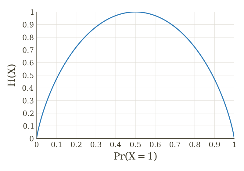
At p = 0 or p = 1, the result is certain and entropy is 0. At p = 0.5, both results are equally likely, so uncertainty is greatest and entropy reaches 1 bit. The curve is symmetric: swapping the two outcomes does not change the entropy.

Five-outcome distributions

Five outcomes with probabilities 0.25, 0.25, 0.25, 0.125, and 0.125. — More balanced: H = 2.25 bits

Five outcomes with probabilities 0.75, 0.0625, 0.0625, 0.0625, and 0.0625. — More concentrated: H ≈ 1.3 bits

p (S) = {0.25, 0.25, 0.25, 0.125, 0.125}

H = 3 \times 0.25 \times \log_{2} 4 + 2 \times 0.125 \times \log_{2} 8 = 1.5 + 0.75 = 2.25 bits

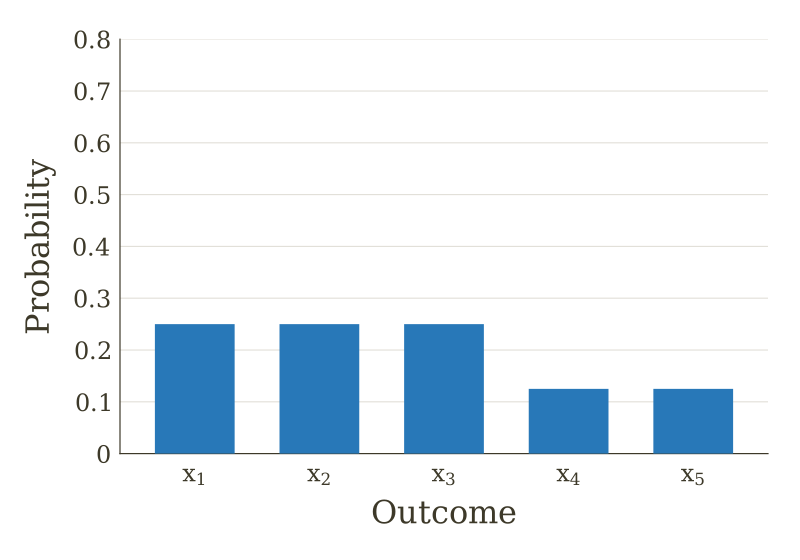
Three outcomes have probability 0.25, giving 2 bits each; two have probability 0.125, giving 3 bits each. The factors 3 and 2 count the repeated probabilities.

p (S) = {0.75, 0.0625, 0.0625, 0.0625, 0.0625}

H = 0.75 \times \log_{2} (\frac{4}{3}) + 4 \times 0.0625 \times \log_{2} 16 \approx 0.3 + 1 = 1.3 bits

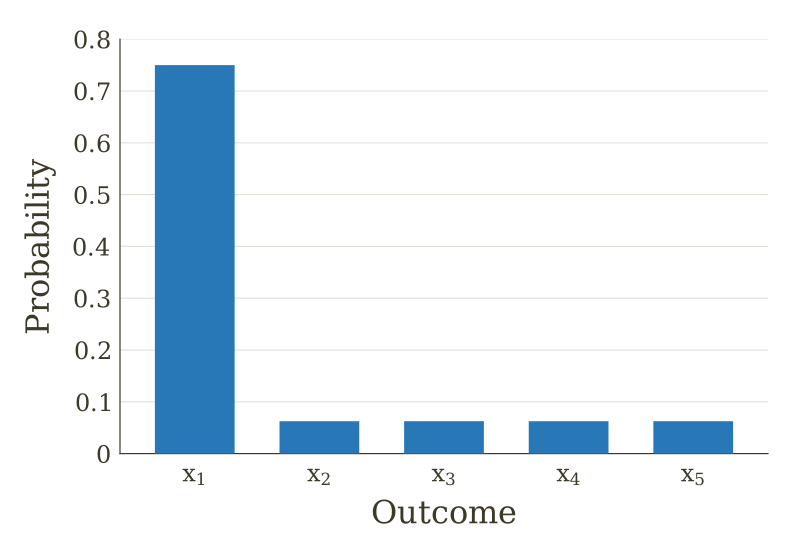
The most likely outcome has probability 0.75, so its information is log₂(4/3). The four rare outcomes each have probability 1/16 and bring 4 bits. The exact entropy is about 1.3113 bits. This distribution is easier to predict because one outcome dominates, so its entropy is lower.

Maximum Entropy MDP

Regular formulation:

max_{π} E [\sum_{t = 0}^{H} r_{t}]

Find the policy π with the highest expected total reward. The sum adds rewards rₜ from time 0 through H, and E averages over the trajectories produced by the policy and the environment. This finite-horizon formula uses undiscounted rewards.

Max-ent formulation:

max_{π} E [\sum_{t = 0}^{H} (\underset{\begin{matrix} ↑ \\ Reward \end{matrix}}{r_{t}} + \underset{\begin{matrix} ↑ \\ Weight \end{matrix}}{β} \underset{\begin{matrix} ↑ \\ Policy entropy \end{matrix}}{ℋ (π (\cdot | s_{t}))})]

At every time step, add an entropy bonus to the reward, then sum both terms over time. This favors policies that earn reward while keeping a more diverse action distribution.

$π (\cdot | s_{t})$ is the full distribution over actions at state sₜ. The dot means all possible actions, rather than one particular action.
$ℋ (π (\cdot | s_{t}))$ applies the entropy formula above to that action distribution. Always choosing one action gives entropy 0; spreading probability more evenly among a fixed set of actions gives higher entropy.
β ≥ 0 controls the weight of the entropy bonus. β = 0 recovers the regular objective. A larger β places more weight on entropy relative to reward; the policy still balances both terms.

H in the sum is the horizon’s last time index; $ℋ$ is the entropy function. They have different meanings.

Example

Consider a one-step task with two actions, each giving reward 1. Always choosing the first action gives entropy 0, so the max-ent objective is 1. Choosing each action with probability 0.5 gives entropy 1 bit, so the objective is 1 + β. With β > 0, the second policy is preferred. If the actions have different rewards, their reward difference also affects the choice.

Max-ent for 1-step problem

The state is fixed and there is one decision. We choose a probability for each action; there are finitely many actions, their rewards are finite, and $β > 0$ .

Here, $log = ln$ , so entropy is measured in nats. Using base-2 logarithms changes the scale of $β$ .

Choose the distribution

$max_{π (a)} E [r (a)] + β ℋ (π (a))$

The unknowns are the action probabilities. The objective balances expected reward with the entropy of their distribution.
Expand reward and entropy

$max_{π (a)} \sum_{a} π (a) r (a) - β \sum_{a} π (a) log π (a)$

Expected reward weights each reward by its action probability. Entropy supplies the second sum. Valid probabilities must satisfy:

$π (a) \geq 0 \forall a, \sum_{a} π (a) = 1$
Enforce normalization

$max_{π (a)} min_{λ} ℒ (π (a), λ) = max_{π (a)} min_{λ} [\sum_{a} π (a) r (a) - β \sum_{a} π (a) log π (a) + λ (\sum_{a} π (a) - 1)]$

$λ$ is a constraint multiplier. It can be any real number: if the probabilities do not sum to 1, it can make the Lagrangian arbitrarily negative. When they sum to 1, its added term is 0.
Differentiate one probability

$\frac{\partial ℒ}{\partial π (a)} = 0$

With positive $β$ , the optimal probabilities are positive. Set the derivative for each action probability to 0, treating the other probabilities and $λ$ as fixed.
Expand the derivative

$\frac{\partial}{\partial π (a)} [\sum_{a} π (a) r (a) - β \sum_{a} π (a) log π (a) + λ (\sum_{a} π (a) - 1)] = 0$

Vary one component $π (a)$ of the distribution. Only that action’s term in each sum changes.
Apply the product rule

$r (a) - β log π (a) \underset{\begin{matrix} ↑ \\ Product rule \end{matrix}}{- β} + λ = 0$

The reward term gives $r (a)$ . Since $\frac{d (x log x)}{d x} = log x + 1$ , the entropy term gives both negative terms. The constraint term gives $λ$ .
Isolate the log probability

$β log π (a) = r (a) - β + λ$

Move the log term to the other side; the same $λ$ applies to every action.
Exponentiate

$π (a) = exp [\frac{1}{β} (r (a) - β + λ)]$

Divide by $β$ , then apply exp to undo the natural logarithm. The factor $C = exp (\frac{λ - β}{β})$ is common to every action.
Differentiate the multiplier

$\frac{\partial ℒ}{\partial λ} = 0$

Only the normalization term contains $λ$ , so this derivative recovers the probability constraint.
Make the probabilities sum to 1

$\sum_{a} π (a) - 1 = 0$

Let $Z$ be the sum of the exponential reward weights. Each weight is multiplied by the same $C$ , so their total probability is $C Z$ . Normalization gives $C Z = 1 \Rightarrow C = \frac{1}{Z}$ .
Normalize the exponential weights

$π (a) = \frac{1}{Z} exp (\frac{1}{β} r (a))$

Divide every positive weight by their common total. The result is a valid action distribution, with higher-reward actions receiving higher probability.
Define the partition function

$Z = \sum_{a} exp (\frac{1}{β} r (a))$

$Z$ is the total exponential weight across all actions. It is positive and finite under the stated assumptions.

For two actions with rewards 1 and 0, $β = 1$ gives probabilities approximately 0.731 and 0.269. A smaller $β$ favors higher-reward actions more strongly; a larger $β$ makes the probabilities more even.

Max-ent for 1-step problem: value

Use the optimal policy derived above, with $β > 0$ and natural logarithms.

π (a) = \frac{1}{Z} \exp (\frac{1}{β} r (a)), Z = \sum_{a} \exp (\frac{1}{β} r (a))

V = \sum_{a} \frac{1}{Z} \exp (\frac{1}{β} r (a)) r (a) - β \sum_{a} \frac{1}{Z} \exp (\frac{1}{β} r (a)) \log [\frac{1}{Z} \exp (\frac{1}{β} r (a))]

Substitute the optimal policy into the reward plus entropy objective. V is the maximized value of this full objective.

V = \sum_{a} \frac{1}{Z} \exp (\frac{1}{β} r (a)) [r (a) - β \log (\exp (\frac{1}{β} r (a)))] - β \sum_{a} \frac{1}{Z} \exp (\frac{1}{β} r (a)) \log (\frac{1}{Z})

Use $\log (u v) = \log (u) + \log (v)$ to split the logarithm, then combine the reward with the exponential term. $\log (\frac{1}{Z})$ is the same for every action.

V = \underset{\begin{matrix} ↑ \\ Reward terms cancel \end{matrix}}{0} - β \log (\frac{1}{Z}) \underset{\begin{matrix} ↑ \\ Probabilities sum to 1 \end{matrix}}{\sum_{a} \frac{1}{Z} \exp (\frac{1}{β} r (a))}

The logarithm reverses the exponential, so $r (a) - β \frac{1}{β} r (a) = 0$ . Pull the remaining constant factor outside the sum.

V = - β \log (\frac{1}{Z})

The probabilities are normalized: $\sum_{a} π (a) = 1$ . The remaining sum therefore becomes 1.

V = β \log \sum_{a} \exp (\frac{1}{β} r (a))

Use $\log (\frac{1}{Z}) = - \log (Z)$ , then replace Z with its defining sum.

The policy probabilities form a softmax distribution. V is a scalar soft maximum: beta times log-sum-exp.

Max-ent Value Iteration

For a finite action set, the one-step solution also works when an action’s score includes the future. Here, β > 0 and log means the natural logarithm.

1. Count the remaining decision steps

Here k counts remaining decision steps; H is the last time index. A sum from time 0 through H contains H + 1 decisions. With no decisions left, the value is 0:

V_{0} (s) = 0

Vₖ(s) is the best expected total reward plus entropy bonus over the last k decisions, starting from state s:

V_{k} (s) = max_{π} E [\sum_{t = H - k + 1}^{H} (r (s_{t}, a_{t}) + β ℋ (π (\cdot | s_{t}))) | s_{H - k + 1} = s]

The expectation averages over action choices and environment transitions. ℋ applies to the full action distribution, and its bonus is included at every decision. In the sum, π denotes a sequence of policies, with π(·|sₜ) meaning the distribution used at time t. Each policy can depend on how many steps remain.

Separate the current decision from the remaining k − 1 decisions:

V_{k} (s) = max_{π} E [r (s, a) + β ℋ (π (\cdot | s)) + V_{k - 1} (s^{'})]

Sample a from π(·|s), then sample s′ from P(·|s,a). The three terms are immediate reward, current entropy bonus, and the best future soft value. Starting from V₀, compute this for k = 1, …, H + 1. This formulation is undiscounted.

2. Define the action value

Q_{k} (s, a) = E [\underset{\begin{matrix} ↑ \\ Reward now \end{matrix}}{r (s, a)} + \underset{\begin{matrix} ↑ \\ Future soft value \end{matrix}}{V_{k - 1} (s^{'})} | s, a]

Fix the current state and action. Only the next-state transition is averaged here. Qₖ includes the current reward and optimal future rewards and entropy bonuses; it leaves the current entropy bonus outside.

3. Reuse the one-step solution

V_{k} (s) = max_{π} E [Q_{k} (s, a) + β ℋ (π (\cdot | s))]

Here max over π chooses the current state’s action distribution; the future is already optimized by Vₖ₋₁. The expectation is only over a ∼ π(·|s). The entropy is the same for every sampled action. Replace the reward score r(s,a) in the one-step derivation with Qₖ(s,a): it already accounts for the optimal soft future.

4. Compute the soft value and policy

V_{k} (s) = β \log \sum_{a} \exp (\frac{1}{β} Q_{k} (s, a))

Ordinary value iteration uses the largest action value, maxₐ Qₖ(s,a). The entropy bonus replaces that maximum with log-sum-exp, which combines all action scores.

π_{k} (a | s) = \frac{1}{Z} \exp (\frac{1}{β} Q_{k} (s, a))

Z = \sum_{a} \exp (\frac{1}{β} Q_{k} (s, a)) = \exp (\frac{V_{k} (s)}{β})

Z depends on s and k and makes the action probabilities sum to 1. Instead of an argmax action, πₖ is a softmax distribution: higher Qₖ gets higher probability. Use πₖ when k steps remain; after one action, k decreases by 1. As β approaches 0 from above, the policy concentrates on greedy actions.

Maximum entropy formulation

What if we could find a distribution over near-optimal solutions?

Entropy

Examples

Binary random variable

Five-outcome distributions

Maximum Entropy MDP

Regular formulation:

Max-ent formulation:

Example

Max-ent for 1-step problem

Choose the distribution

Expand reward and entropy

Enforce normalization

Differentiate one probability

Expand the derivative

Apply the product rule

Isolate the log probability

Exponentiate

Differentiate the multiplier

Make the probabilities sum to 1